 Population structure analysis is a statistical method used to infer the genetic composition and ancestry proportions of individuals within a population. This type of study allows us to understand genetic variation within and between populations. Building admixture models provides insights into evolutionary processes, migration patterns, and even disease susceptibility. ADMIXTURE, now available in OmicsBox, makes this analysis easier by providing a step-by-step walkthrough.
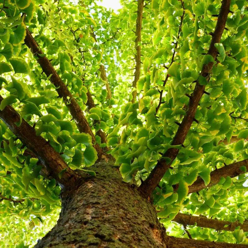
In this blog, we will analyze the population structure of Ginkgo samples from start to finish, demonstrating how to use OmicsBox to conduct this type of analysis with ADMIXTURE.
Data Description
- 102 Ginkgo samples were downloaded from the Chinese National Genomics Data Center with Accession Number CRA006613. This data was originally used in Y. Hu et al. (2023).
- Paired-end FASTQ files of 3GB approx. per sample.
- FASTQ files were obtained using a GBS methodology.
- Ginkgo Biloba possesses one of the largest genomes with approximately 11.5 Gb in size.
- Ginkgo Biloba reference genome was downloaded from the Chinese National Genomics Data Center.
Methodology
All tools mentioned here are part of OmicsBox. The first step is part of the genome analysis module, whereas the rest requires the genetic variation module:
- FASTQ files were downloaded and mapped to the reference Ginkgo genome using BWA with default parameters. The resulting alignments were returned in BAM file format.
- The BAM files and the same reference genome were used as input in BCFtools with default parameters in order to obtain a preliminary VCF file. This raw VCF file will contain all variants found by BCFtools, regardless of their quality.
- Then, this VCF file was filtered in order to remove unreliable variants and reduce the size of the dataset.
- This filtered VCF file was phased and imputed using Beagle by default parameters in order to estimate genotypes that might have not been called by BCFtools.
- After an intermediate step of Linkage Disequilibrium pruning (LD pruning) using BCFtools, Population Structure Analysis was performed using ADMIXTURE.
Population Structure Results in OmicsBox
Once the Population Structure Analysis is complete, OmicsBox will display the following results.
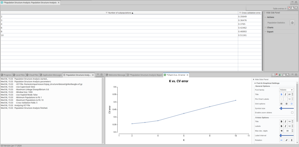
The output will display a table containing estimated models and their Cross Validation (CV) errors, a summary report and a chart depicting this information. The models will vary based on the number of subpopulations (K) present in the VCF file population.
Selecting a Suitable Model
The plot representing each model and the CV error looks like this:
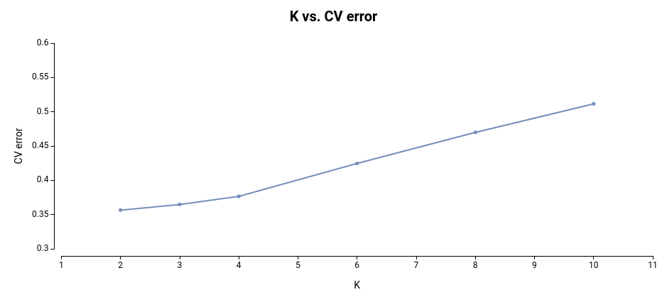
As observed, the most effective models for this dataset are those built on 2 and 3 subpopulations, as they exhibit the lowest cross-validation error.
Differences between Samples
Doing a Principal Component Analysis (PCA) from a VCF file is really useful to see how your samples differ. A PCA can be done in a VCF file by maximizing the variance of the genotypes across samples. Furthermore, we will color each sample in the PCA plot according to the corresponding subpopulation they belong to following the results of ADMIXTURE in OmicsBox.
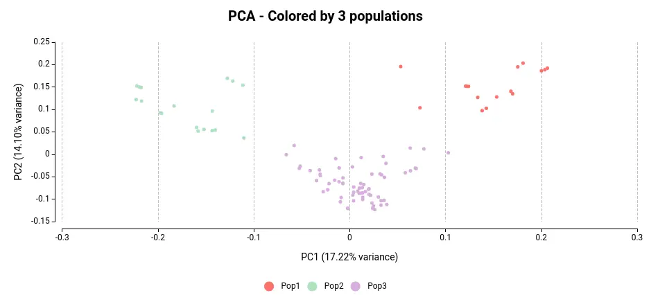
Regardless of the color, we can see that the samples in the VCF file are organized into three distinct clusters. By assigning colors to the samples based on their subpopulation as determined by the population structure analysis (see Figure 3), we can observe that each cluster corresponds to a unique population.
Differences between Subpopulations
In OmicsBox, you will be able to plot a heatmap of the Fst among subpopulations. Fst is a measure of the genetic distance between two subpopulations. The higher the value of Fst, the greater the difference between subpopulations. Here we have the heatmap depicting this variability among these 3 subpopulations:
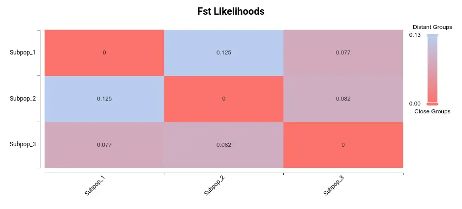
The most significant difference appears to be between subpopulations 1 and 2. Upon examining the PCA plot in Figure 3, it becomes apparent that Populations 1 and 2 exhibit the greatest separation.
Population Genetics Statistics
Different population statistics can provide insights into the origins and tendencies of subpopulations. In OmicsBox, you can find the following:
- Tajima’s D: This test helps distinguish a population following the Hardy-Weinberg equilibrium (value close to 0) from a changing population.
- Pi (π): Also known as nucleotide diversity, this variable is a measure of genetic variation.
- Heterozygosity: This represents the fraction of heterozygous variants in the total number of variants.
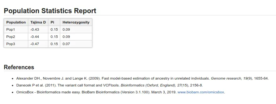
As can be seen in Figure 4 and Figure 5, the three populations are not very different. In Figure 4, we see that Fst values are not very high (max. value is 0.125), and in Figure 5 we cannot see great differences in population statistics.
However, despite their close relationship, ADMIXTURE has identified a model in which 3 subpopulations successfully detect in this ginkgo dataset.
Conclusions
- You can use ADMIXTURE to find subtle subpopulations in a set of samples in the VCF file.
- OmicsBox enables the complete workflow from DNA sequencing to population analysis passing through variant calling, filtering, phasing and imputation of variants.
- The user-friendly wizards and the additional information provided by OmicsBox help your research studies throughout the process.
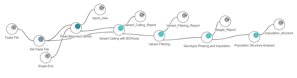
Figure 6. Workflow used in OmicsBox
References
Hu, Y., Yu, Z., Gao, X., Liu, G., Zhang, Y., Šmarda, P., & Guo, Q. (2023). Genetic diversity, population structure, and genome-wide association analysis of ginkgo cultivars. Horticulture Research, 10(8), uhad136.
Liu, H., Wang, X., Wang, G., Cui, P., Wu, S., Ai, C., … & Cao, F. (2021). The nearly complete genome of Ginkgo biloba illuminates gymnosperm evolution. Nature Plants, 7(6), 748-756.
Li H. and Durbin R. (2009) Fast and accurate short read alignment with Burrows-Wheeler transform. Bioinformatics, 25, 1754-1760. [PMID: 19451168]. (if you use the BWA-backtrack algorithm)
B L Browning, X Tian, Y Zhou, and S R Browning (2021) Fast two-stage phasing of large-scale sequence data. Am J Hum Genet 108(10):1880-1890. doi:10.1016/j.ajhg.2021.08.005
B L Browning, Y Zhou, and S R Browning (2018). A one-penny imputed genome from next generation reference panels. Am J Hum Genet 103(3):338-348. doi:10.1016/j.ajhg.2018.07.015
Deschamps, S., Llaca, V., & May, G. D. (2012). Genotyping-by-sequencing in plants. Biology, 1(3), 460-483.
D.H. Alexander, J. Novembre, and K. Lange. Fast model-based estimation of ancestry in unrelated individuals. Genome Research, 19:1655–1664, 2009.

About the Author

With a biological and technological academic background, including a BSc in Biotechnology and an MSc in Bioinformatics, Enrique’s expertise lies in the areas of Long Reads and Genetic Variation.