Pairwise Differential Expression Analysis

A simple use-case comparing OmicsBox with R chunks

The OmicsBox feature “Pairwise Differential Expression Analysis” is designed to perform differential expression analysis of count data arising from RNA-seq technology. This tool allows the identification of differential expressed genes considering two different conditions based on the software package ‘edgeR’, which belongs to the Bioconductor project. This use case shows the basic analysis workflow, comparing the results obtained with R Bioconductor and OmicsBox.

DataSet

This analysis describes a differential expression analysis of an RNA-Seq dataset from tomato (Solanum lycopersicum) pollen undergoing chronic heat stress. Samples and counts were obtained from the laboratory of Nurit Firon. The control plants (C1-C5) were grown at 28/18 ºC and the treatment samples (T1-T5) were grown at 32/26 ºC day/night. Each collection includes one treatment and one control sample consisting of pollen pooled from multiple plants.

Download:

• experimental_design.txt
• count_table.txt

Video tutorial:

• How to perform a Pairwise Differential Expression Analysis using OmicsBox

Analysis Workflow

1. Loading Data

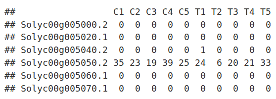
The read counts for the ten individual libraries were stored in one tab-delimited file. EdgeR only accepts raw counts without any type of normalization.

library(edgeR)

rawdata=read.delim('/data/tomato_counts.txt', 
    check.names=F, stringAsFactors=F, 
    row.names=1)

group=c('C','C','C','C','C',
    'T','T','T','T','T')

dge=DGEList(rawdata, group=group)

OmicsBox:  The file containing the count table is loaded: File → Load → Load Count Table. Note that the data are nicely formatted, with gene names as row names and sample names as column names.

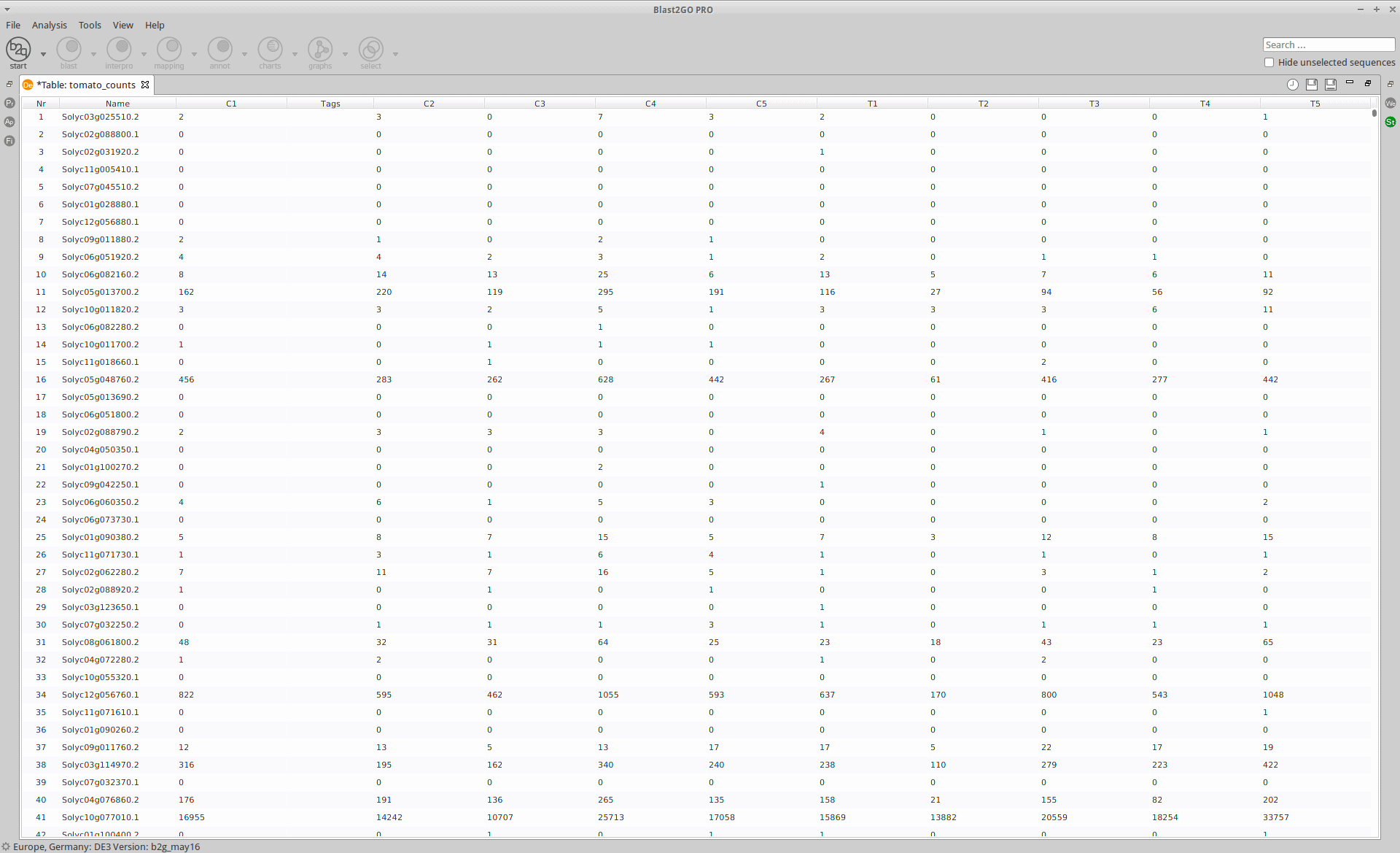2. Filtering and Normalization

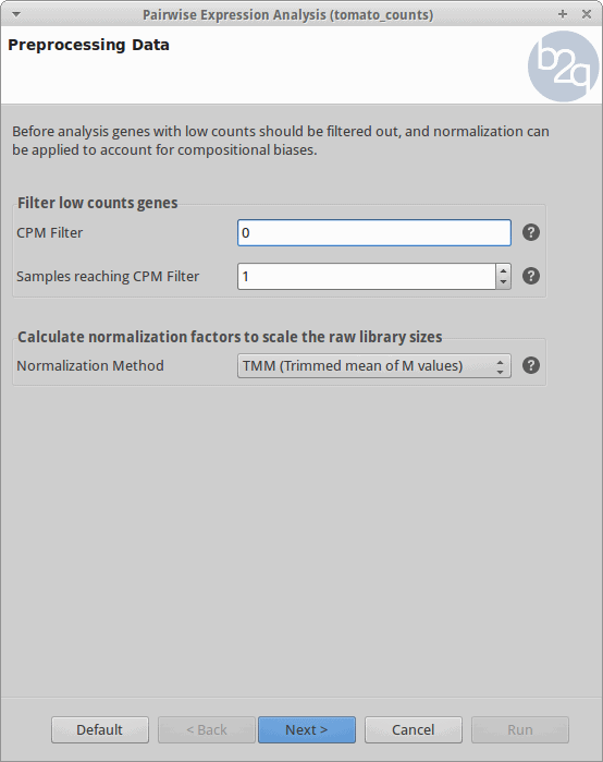
Genes with zero counts are eliminated since it makes no sense to test them for differential expression if they were not expressed. Normalization is applied to account for compositional difference between the libraries. Note that when normalization is applied in edgeR, the software does not change the counts. Instead, it calculates normalization factors that will be used later.

##Filtering
keep=rowSums(cpm(dge) > 0) >= 1
dge=dge[keep, , keep.lib.sizes=F]

##Normalization
dge=calcNormFactors(dge, method='TMM')

OmicsBox:  The adjustment of filtering and normalization steps is performed on the “Preprocessing Data” page of the main wizard: Diff Exprs → Run Differential Expression Analysis (“Pairwise Differential Expression Analysis” option).

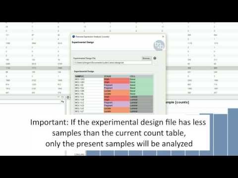
3. Experimental Design

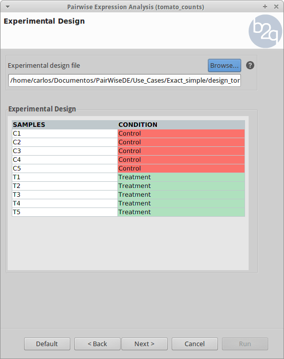
The experimental design of this case corresponds to two experimental conditions, “Control” and “Treatment”, with five replicates each one.

groups = c('C','C','C','C','C',
        'T','T','T','T','T')
dge$samples = groups

OmicsBox:  On the “Experimental Design” page of the main wizard, users can load the experimental design of their data.

4. Comparison and Test

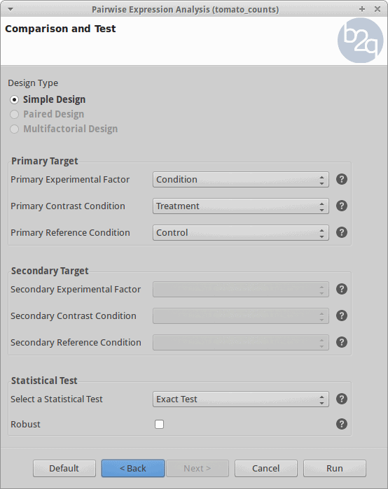
For the analysis, all the control and treatment samples will be treated as replicates in order to identify genes whose expression changed due to the heat stress treatment. This corresponds to what the edgeR manual calls the “classic approach” (Exact test).

##Dispersions
dge=estimateDisp(dge)

##Test
dex=exactTest(dge, pair=c('C','T'))

OmicsBox:  On the “Comparison and Test” page of the main wizard, users can choose the experimental conditions to compare and select the statistical test.

Results

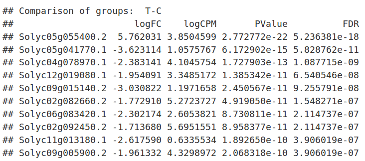
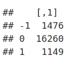
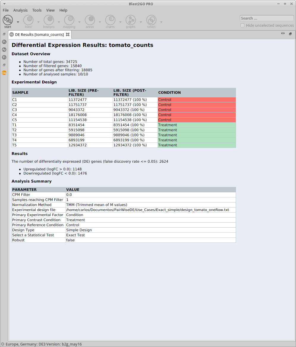
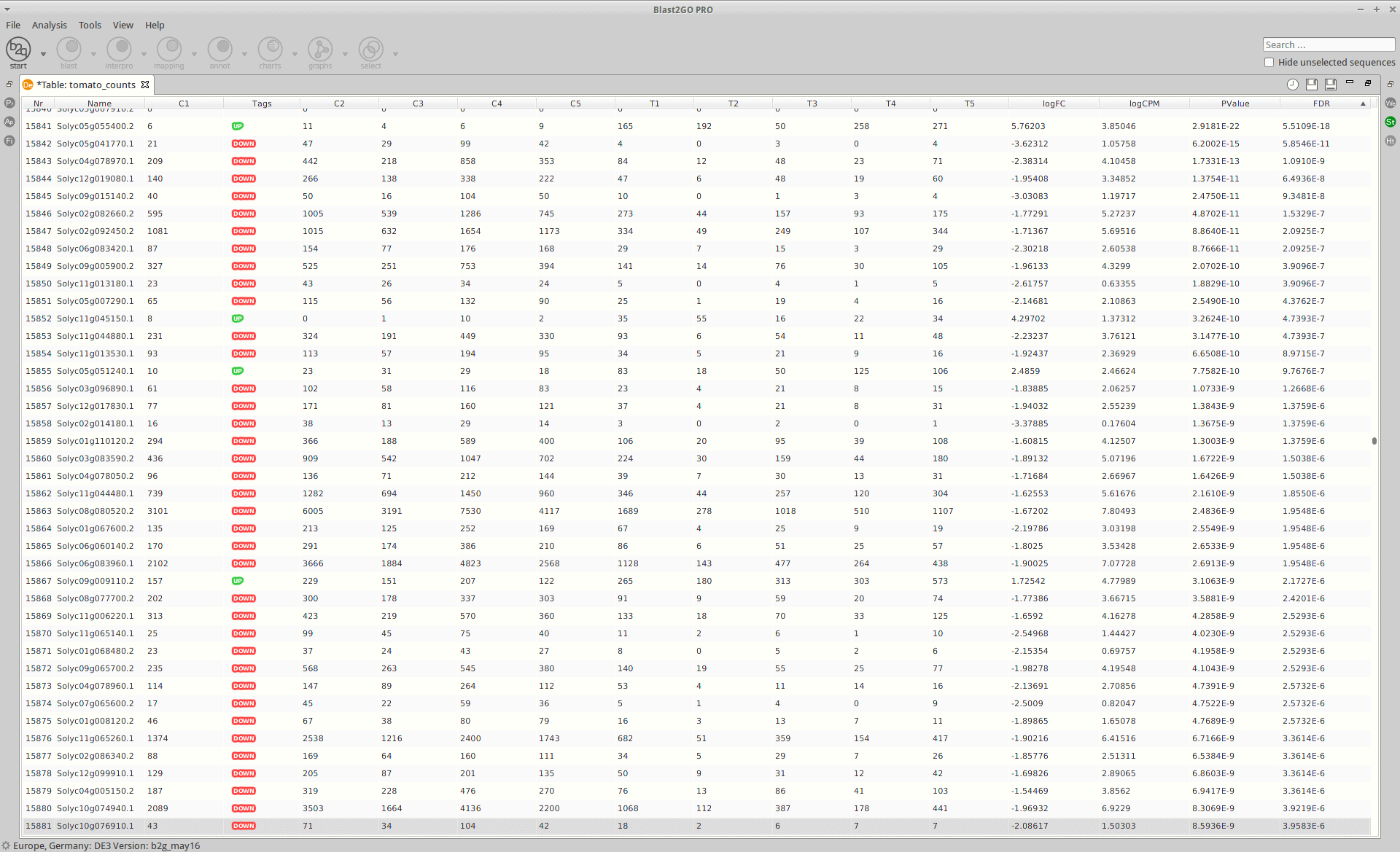
After the analysis, interpretation of results is important to reach biological conclusions.

TopTags(dex)

summary(decideTestsDGE(dex, p=0.05))

OmicsBox:  Once the input counts has been processed and analyzed, results will be displayed on the Main Generic Table Viewer.

A result page shows a summary of the differential expression analysis results.

Statistics

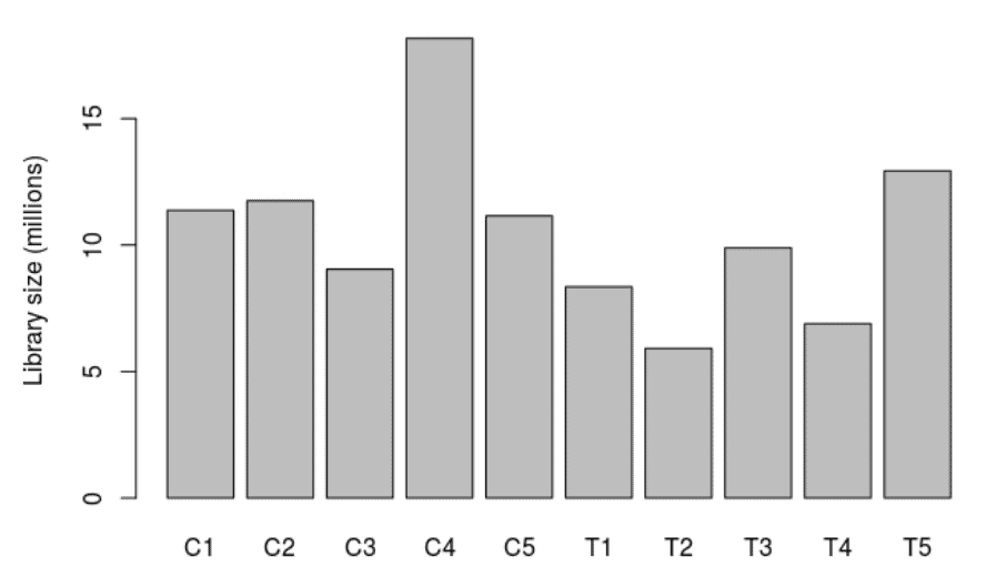
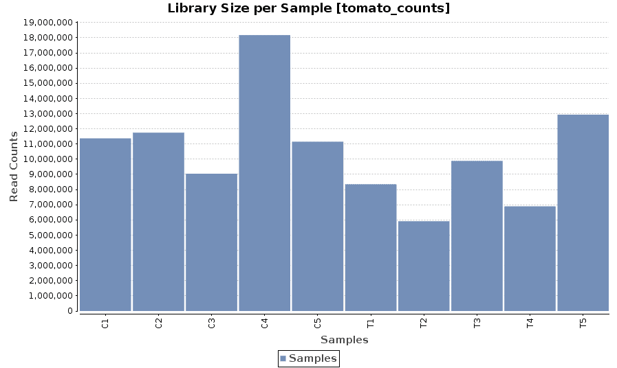
1. Library Size

A bar chart showing the read counts contained in each sample.

barplot(dge$samples$lib.size*1e-6,
    names=colnames(dge$counts),
    ylab='Library size (millions)')

OmicsBox:  Diff Expr → View Results: Pairwise Analysis → Statistics → Library Size per Sample.

2. MDS Plot

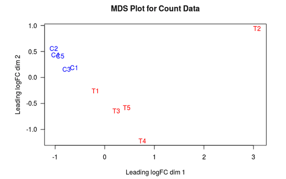
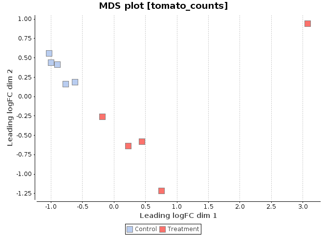
A multi-dimensional scaling (MDS) plot can show similarity between samples in which distances correspond to leading log-fold-changes between each pair of RNA samples. The leading log-fold-change is the average (root-mean-square) of the largest absolute log-fold-changes between each pair of samples. This plot can be viewed as a type of unsupervised clustering.

cn.color='blue'
tr.color='red'
main='MDS Plot for Count Data'
par(las=1)
colors=c(rep(cn.color,5),rep(tr.color,5))
plotMDS(dge, main=main, 
    labels=colnames(dge$counts), 
    col=colors, las=1)

OmicsBox:  Diff Expr → View Results: Pairwise Analysis → Statistics → MDS Plot.

3. MA Plot

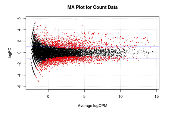
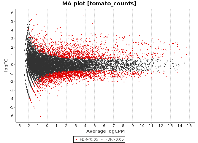
This chart illustrates the relationship between logFC and average expression level for the differential expressed genes, which are highlighted in red. The blue lines indicate genes that are up or down-regulated two fold.

de=decideTestsDGE(dex, p=0.05, adjust='BH')
detags=rownames(dex)[as.logical(de)]
plotSmear(dex, de.tags=detags, 
    main='MA Plot for Count Data')
abline(h=c(-1,1), col='blue')

OmicsBox:  Diff Expr → View Results: Pairwise Analysis→ Statistics → MA Plot.

4. Volcano Plot

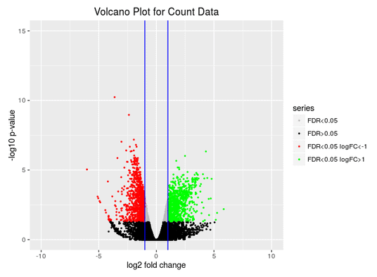
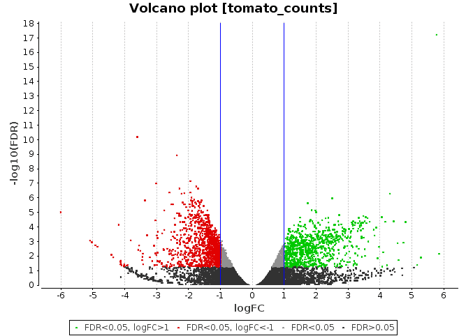
Scatter chart that is constructed by plotting the negative log of the adjusted p-values (FDR) on the y-axis versus the log of the fold changes on the x-axis.

libarary(ggplot2)
ggplot(data=results, aes(x=logFC, 
        y=-log10(FDR), colour=series))+
    geom_point(size=0.5)+
    xlim(c(-10,10))+
    ylim(c(0,15))+
    xlab('log2 fold change')+
    ylab('-log10 p-value')+
    scale_color_manual(values=
        c('gray', 'black', 'red', 'green'))+
    ggtitle('Volcano Plot for Count Data')

OmicsBox:  Diff Expr → View Results: Pairwise Analysis → Statistics → Volcano Plot.

Conclusions

As shown in this use case, the edgeR package is a powerful tool that allows statistical analysis for RNA-seq technology data.  The OmicsBox feature “Pairwise Differential Expression Analysis” uses all the edgeR statistical potential to offer an easy and simple way to perform this type of analysis, without requiring programming skills. Futhermore, users can take advantage of OmicsBox features to complete the analysis and achieve greater understanding of the biological problem that is being studied.

References:

Robinson MD, McCarthy DJ and Smyth GK (2010). “edgeR: a Bioconductor package for differential expression analysis of digital gene expression data.” Bioinformatics, 26, pp. -1.